Functional-Based Reserving with the R Package ProfileLadder

The R package ProfileLadder provides nonparametric, functional-based methods for claims reserving based on aggregated chain-ladder data also known as the run-off triangles. The package implements three estimation/prediction algorithms (PARALLAX, REACT, and MACRAME) and the permutation bootstrap add-on proposed in Maciak, Mizera, and Pešta (2022).

The package offers a flexible and computationally effective framework for point-wise and distributional reserve predictions and includes pertinent visualization and diagnostic tools through standard S3 methods—such as plot(), predict(), print(), or summary(). It also provides accessor functions and real-world datasets to support exploratory analysis across insurance, operational risks, and other domains where triangular data structures arise, making modern, transparent, and extensible alternatives to classical approaches accessible in insurance industry and academic research.

The following lines provide an illustrative sample analysis and reserve prediction for two specific run-off triangles using all three nonparametric prediction algorithms and other functions introduced within the ProfileLadder package. The functionality of the core functions of the package are and some important features are presented and discussed. Further theoretical details can be found in

Maciak, M., Mizera, I., and Pešta, M. (2022). Functional Profile Techniques for Claims Reserving. ASTIN Bulletin, 52(2), 449 – 482. DOI: 10.1017/asb.2022.4

Package manual and GitHub pages

PDF/HTML manual: https://CRAN.R-project.org/package=ProfileLadder
GitHub Pages: https://42463863.github.io/ProfileLadder/index.html

The package ProfileLadder can be installed directly from CRAN using a standard command

install.packages("ProfileLadder")

The package ProfileLadder also allows for a convenient and elegant integration with the leading actuarial R package ChainLadder commonly utilized for risk assessment and actuarial practice. This is mainly ensured through two functions implemented in ProfileLadder, as.profileLadder() and observed(). Therefore, both these actuarial libraries (R packages) are used in the following illustrations.

library("ProfileLadder")
library("ChainLadder")

Package structure

The key functions of the ProfileLadder package that implement three functional-based nonparametric (point) reserve prediction algorithms and the overall (distributional) reserve prediction in terms of the proposed permutation bootstrap resampling are

parallelReserve() – for PARALLAX and REACT;
mcReserve() – for the MACRAME algorithm;
permuteReserve() – for the permutation bootstrap add-on.

Note some obvious (and practically convenient) similarities of the notation and the implementation details that shared with the R package ChainLadder. More details about the package structure—all functions, S3 type methods, accessor functions, and illustrative datasets can be found on GitHub Pages.

Notation and example datasets

There are two real datasets—cumulative run-off triangles (both from the package ProfileLadder)—used in the following claims reserving example.

The cummulative run-off triagle is a specific data structure represented by a collection of random variables denoted as $\{Y_{i,j};~i = 1, \dots, n; j = 1, \dots, n - i + 1\}$ , where the rows $\{(Y_{i. 1}, \dots, Y_{i, n - i + 1})\}_{i = 1}^n$ are typically assumed to be independent among each other and they represent the origins of the reported claims. The columns, on the other hand, represent the development periods.

The incremental run-off triagle is an analogous dataset represented by a collection of random variables $X_{i,j}$ ’s, $\{X_{i,j};~i = 1, \dots, n; j = 1, \dots, n - i + 1\}$ , where $X_{i,j} = Y_{i,j} - Y_{i, j - 1}$ , for $i \in \{1, \dots, n\}$ and $j = 1, \dots, n - i + 1$ , where, in addition, $Y_{i,0} = 0$ for completeness.

There are numerous (real-life) datasets (run-off triangles) not only from the actuarial practice provided as an integral part of the ProfileLadder package while most of them were not yet made available in any other R package nor any other publicly available source. Some of the datasets are unique in this aspect: For instance, the dataset GFCIB, provided by the Guarantee Fund of the Czech Insurers’ Bureau (GFCIB) and datasets CZ.casco, CZ.liability, and CZ.property provided by a major and market-leading insurance company in the Czech Republic contain relatively large (compared to other publicly available actuarial data) run-off triangles (for example, GFCIP from the mandatory car insurance in the Czech Republic contains $60$ origins/quarters and $60$ development periods—quarters again). Similarly, the datasets CZ.casco, CZ.liability, and CZ.property provide separate run-off triangles for gross paid amounts and RBNS reserves (all with the dimensions $17 \times 17$ years).

A comprehensive overview of the data included in the ProfileLadder package can be obtained in a standard way by using the command

data(package = "ProfileLadder")

Two particular run-off triangles are selected in the following illustrations:

a) Cameron Mutual Insurance Company Data

The dataset belongs to a larger database of real run-off triangles (provided by Mayers and Shi, 2011) and available also (in a long format structure) in the R package raw. The run-off triangle is completed into a full square—meaning that “future” payments are known (typically they are provided retrospectively, mainly for some evaluation and back-testing purposes). `

help("CameronMutual") ## output omitted
(cameron <- CameronMutual)

##       dev
## origin    1     2     3     4     5     6     7     8     9    10
##     1  5244  9228 10823 11352 11791 12082 12120 12199 12215 12215
##     2  5984  9939 11725 12346 12746 12909 13034 13109 13113 13115
##     3  7452 12421 14171 14752 15066 15354 15637 15720 15744 15786
##     4  7115 11117 12488 13274 13662 13859 13872 13935 13973 13972
##     5  5753  8969  9917 10697 11135 11282 11255 11331 11332 11354
##     6  3937  6524  7989  8543  8757  8901  9013  9012  9046  9164
##     7  5127  8212  8976  9325  9718  9795  9833  9885  9816  9815
##     8  5046  8006  8984  9633 10102 10166 10261 10252 10252 10252
##     9  5129  8202  9185  9681  9951 10033 10133 10182 10182 10183
##     10 3689  6043  6789  7089  7164  7197  7253  7267  7266  7266

b) Vehicles Damages within a Conventional Full Casco Insurance

The second dataset represents a standard run-off triangle as it is typically available for actuaries when performing the risk assessment task and predicting the point and distributional reserve. The dataset represents cumulative payments for claims related to the compulsory vehicle insurance in the Czech Republic (having 17 origin years and, similarly, 17 development perios—years again).

help("CZ.casco") ## output omitted
(casco <- CZ.casco$GrossPaid)

##       dev
## origin    Dev1    Dev2    Dev3    Dev4   Dev5   Dev6   Dev7   Dev8   Dev9
##     1   532522  689585  688841  689149 689357 689775 689742 689851 689851
##     2   423582  522523  522135  522605 522643 522352 522352 522329 522314
##     3   373866  486702  487670  486499 486370 486335 486352 486352 486260
##     4   441769  561423  558395  557759 557882 558181 558096 557934 557847
##     5   503292  632003  630153  630124 629686 629598 630431 630378 630357
##     6   554625  699257  700824  700508 700930 700889 701568 701462 701452
##     7   613011  759145  759427  759916 758478 758380 758204 758097 758324
##     8   605922  754837  758541  760264 760850 761308 761178 761153 761108
##     9   555154  659550  662410  663053 667075 667300 669785 669770 670158
##     10  514900  622015  623098  624337 624632 624664 624664 626112     NA
##     11  581196  706328  708099  708853 708447 708194 708428     NA     NA
##     12  613266  778185  780959  781436 781720 781561     NA     NA     NA
##     13  706120  885442  890414  891789 894514     NA     NA     NA     NA
##     14  859707 1052701 1057512 1059593     NA     NA     NA     NA     NA
##     15  951189 1197280 1207771      NA     NA     NA     NA     NA     NA
##     16 1061511 1317965      NA      NA     NA     NA     NA     NA     NA
##     17 1121591      NA      NA      NA     NA     NA     NA     NA     NA
##       dev
## origin  Dev10  Dev11  Dev12  Dev13  Dev14  Dev15  Dev16  Dev17
##     1  689839 689813 689795 689767 689664 689613 689568 689497
##     2  522271 522267 522231 522196 522104 522072 522003     NA
##     3  486090 485992 485988 485984 485984 485984     NA     NA
##     4  557781 557588 557198 557062 557049     NA     NA     NA
##     5  630338 630280 630270 630271     NA     NA     NA     NA
##     6  701439 701433 701433     NA     NA     NA     NA     NA
##     7  758263 758233     NA     NA     NA     NA     NA     NA
##     8  761068     NA     NA     NA     NA     NA     NA     NA
##     9      NA     NA     NA     NA     NA     NA     NA     NA
##     10     NA     NA     NA     NA     NA     NA     NA     NA
##     11     NA     NA     NA     NA     NA     NA     NA     NA
##     12     NA     NA     NA     NA     NA     NA     NA     NA
##     13     NA     NA     NA     NA     NA     NA     NA     NA
##     14     NA     NA     NA     NA     NA     NA     NA     NA
##     15     NA     NA     NA     NA     NA     NA     NA     NA
##     16     NA     NA     NA     NA     NA     NA     NA     NA
##     17     NA     NA     NA     NA     NA     NA     NA     NA

1. Data visualization with `ProfileLadder`

Run-off triangles can be either printed in terms of a complete/incomplete matrix (as above) or the data can be visualized using a standard plot() method; however, two different S3 classes for the underlying run-off triangle can be used—the run-off triangle is either of the class triangle (the S3 class provided by the actuarial package ChainLadder) or an extented triangle class profileLadder, implemented in the R package ProfileLadder, can be used as a more complex alternative:

par(mfrow = c(1,2))

### S3 class 'triangle' from the ChainLadder pkg
plot(as.triangle(casco))

### S3 class 'profileLadder' from the ProfileLadder pkg
plot(as.profileLadder(casco))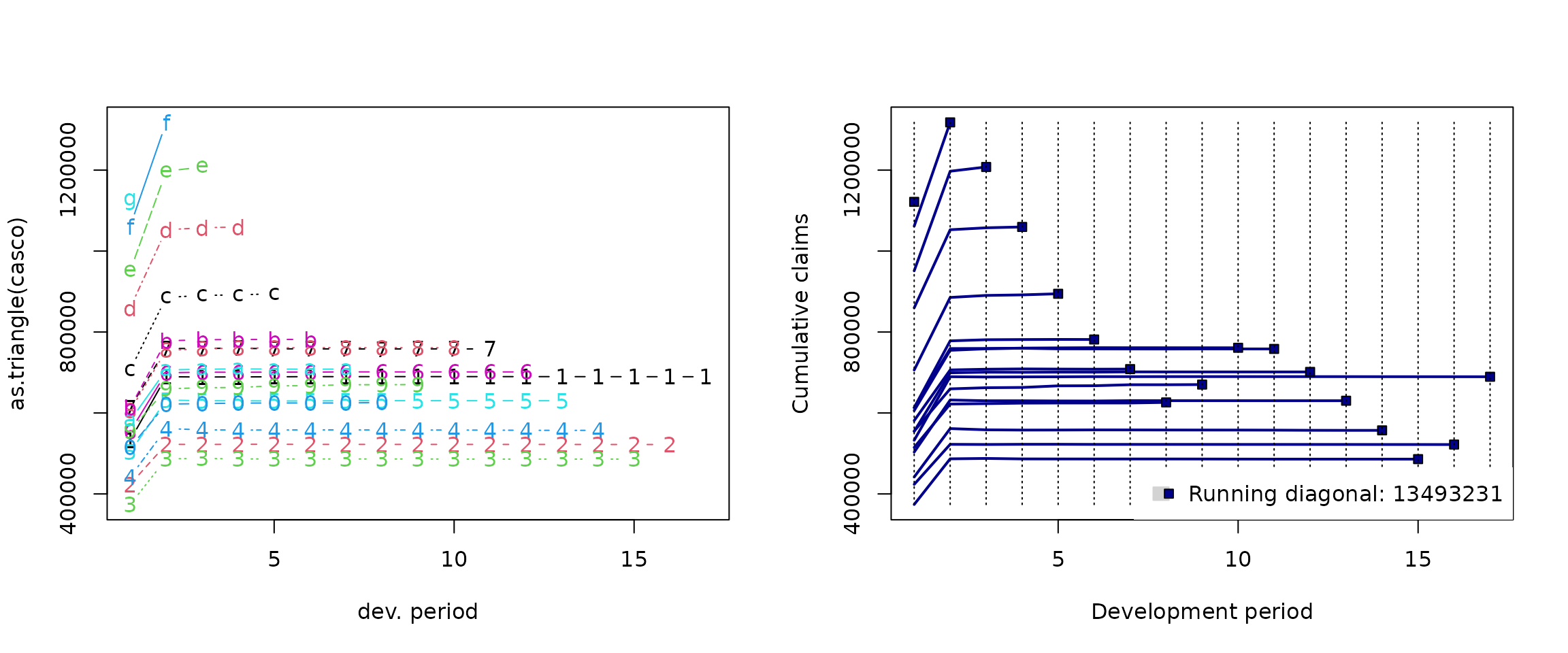

The extended triangle class ProfileLadder (which can be converted from the S3 classes triangle or matrix by using the as.profileLadder() function) allows, in addtion, for plotting the future (“unknown”) profiles—if they are provided in the data for some comparisons, back-testing, or other evaluation purposes. This can be illustrated for the Cameron Mutual insurance data (that contain such future profiles):

par(mfrow = c(1,3))
### S3 class 'triangle' from the ChainLadder pkg
plot(as.triangle(cameron))

### S3 class 'profileLadder' from the ProfileLadder pkg 
plot(as.profileLadder(observed(cameron)))

### S3 class 'profileLadder' (run-off triangle with future profiles)
plot(as.profileLadder(cameron))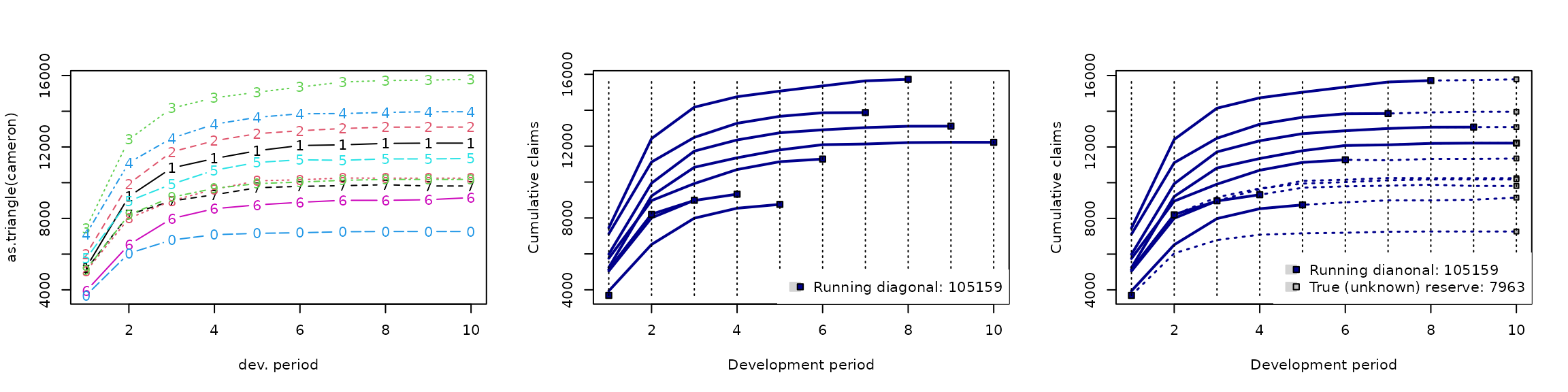

Once the future profiles are provided in the data, the information about the true reserve, typically denoted as $R$ and defined as $R = \sum_{i = 1}^n Y_{i, n} - \sum_{i = 1}^n Y_{i, (n - i + 1)},$ is also reflected in the legend as True (unknown) reserve (see the right panel in the figure above). Otherwise, the task of an actuary is to predict the reserve as $\widehat{R} = \sum_{i = 2}^n \widehat{Y}_{i, n} - \sum_{i = 2}^n Y_{i, (n - i + 1)},$ where $\widehat{Y}_{i, n}$ for $i = 2, \dots, n$ represents the predicted ultimate payments (the last column of the completed run-off triangle). The quantity $\sum_{i = 1}^n Y_{i, (n - i + 1)}$ represents the amount of already paid claims (the sum of the last running diagonal, values $Y_{i, n - i + 1}$ , for $i = 1, \dots, n$ ).

Note: The utility function observed(), used in the code above and implemented in the R package ProfileLadder, allows an easy integration of the package with the core actuarial library ChainLadder and, particularly, the easily use the data from other R package raw in both parametric and nonparametric reserving techniques. More details can be found using the R help session help("observed").

2. PARALLAX

The idea of the PARALLAX algorithm (PARALLel ApproXimation of missing fragments), is to impute the missing parts of the run-off triangle by the most similar segments—triangle rows that can be found among the already observed development profiles. The name reflects the fact that the imputation of missing segments in unobserved functional development profiles is always performed in a parallel way using the observed fragments.

To illustrate the principle, we use the Cameron Mutual data first. The run-off triangle provides also the “unknown” future outcomes (functional profile segments that are supposed to be predicted by the algorithm). However, typical information used in the actuarial practice (for claims reserving and reserve prediction) would be of the run-off triangle form as

observed(cameron)

##       dev
## origin    1     2     3     4     5     6     7     8     9    10
##     1  5244  9228 10823 11352 11791 12082 12120 12199 12215 12215
##     2  5984  9939 11725 12346 12746 12909 13034 13109 13113    NA
##     3  7452 12421 14171 14752 15066 15354 15637 15720    NA    NA
##     4  7115 11117 12488 13274 13662 13859 13872    NA    NA    NA
##     5  5753  8969  9917 10697 11135 11282    NA    NA    NA    NA
##     6  3937  6524  7989  8543  8757    NA    NA    NA    NA    NA
##     7  5127  8212  8976  9325    NA    NA    NA    NA    NA    NA
##     8  5046  8006  8984    NA    NA    NA    NA    NA    NA    NA
##     9  5129  8202    NA    NA    NA    NA    NA    NA    NA    NA
##     10 3689    NA    NA    NA    NA    NA    NA    NA    NA    NA

A fancy print option is also implemented in the ProfileLadder package to visually distinguish between the data part that is typically available at the time of the reserve prediction and the data that are provided ex-post for some evaluation purposes. This can be set or altered (in the interactive environments only) by

options(profileLadder.fancy = TRUE) 
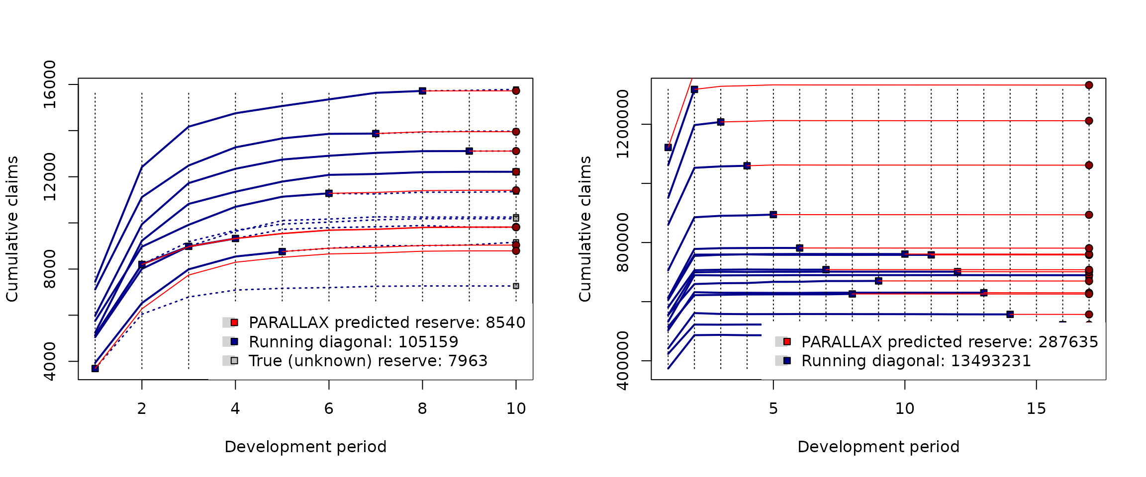
set.fancy.print() ## custom-defined colors

The prediction of the future claims performed by the PARALLAX algorithm is obtained as

(parallax.cameron <- parallelReserve(cameron))

## PARALLAX Reserving 
##     Estimated Reserve    Estimated Ultimate           Paid Amount 
##                  8540                113699                105159 
##          True Reserve 
##                  7963

## PARALLAX method (functional profile completion)

## 5244      9228   10823   11352   11791   12082   12120   12199   12215   12215   
## 5984      9939   11725   12346   12746   12909   13034   13109   13113   13113   
## 7452     12421   14171   14752   15066   15354   15637   15720   15724   15724   
## 7115     11117   12488   13274   13662   13859   13872   13947   13951   13951   
## 5753      8969    9917   10697   11135   11282   11320   11399   11415   11415   
## 3937      6524    7989    8543    8757    8904    8942    9021    9037    9037   
## 5127      8212    8976    9325    9539    9686    9724    9803    9819    9819   
## 5046      8006    8984    9333    9547    9694    9732    9811    9827    9827   
## 5129      8202    8966    9315    9529    9676    9714    9793    9809    9809   
## 3689      6276    7741    8295    8509    8656    8694    8773    8789    8789

As far as the input data also contains “unknown” future developments, the output above also provides the amount of the true reserve (7963 – which is not printed otherwise). Standard summary method can be applied to the output of the parallelReserve() function – the S3 object of the class ProfileLadder:

summary(parallax.cameron)

## PARALLAX reserve prediction (by origins)
##       First Latest Dev.To.Date Ultimate IBNR
## 2      5984  13113   1.0000000    13113    0
## 3      7452  15720   0.9997456    15724    4
## 4      7115  13872   0.9943373    13951   79
## 5      5753  11282   0.9883487    11415  133
## 6      3937   8757   0.9690163     9037  280
## 7      5127   9325   0.9496894     9819  494
## 8      5046   8984   0.9142159     9827  843
## 9      5129   8202   0.8361709     9809 1607
## 10     3689   3689   0.4197292     8789 5100
## total 49232  92944   0.9158488   101484 8540

## Overall reserve summary

##     Est.Reserve    Est.Ultimate     Paid Amount    True Reserve        Reserve% 
##         8540.00       113699.00       105159.00         7963.00            7.25

The summary output above is analogous to the output provided by parametric reserving methods implemented in ChainLadder. For example, considering a typical benchmark over-dispersed Poisson model (ODP) implemented in glmReserve() from the R package ChainLadder, the following summary output is provided:

summary(glmReserve(observed(cameron)))

##       Latest Dev.To.Date Ultimate IBNR          S.E        CV
## 2      13113   1.0000000    13113    0   0.01035287       Inf
## 3      15720   0.9992372    15732   12  29.38975320 2.4491461
## 4      13872   0.9934116    13964   92  73.46098788 0.7984890
## 5      11282   0.9850694    11453  171  96.26787355 0.5629700
## 6       8757   0.9688019     9039  282 120.58781735 0.4276164
## 7       9325   0.9397360     9923  598 177.57019068 0.2969401
## 8       8984   0.8905630    10088 1104 246.00693847 0.2228324
## 9       8202   0.7789914    10529 2327 379.54811405 0.1631062
## 10      3689   0.4788422     7704 4015 622.22022041 0.1549739
## total  92944   0.9152986   101545 8601 880.66723938 0.1023913

Due to obvious analogy between the outputs from the nonparametric reserving method (‘parallelReserve()’) and the standard parametric approach (glmReserve()) we omit further interpretation of the whole output and we only focuss on differences.

Note: The outout from the summary() method applied to the S3 class object profileLadder produced by the parallelReserve() function from the R package ProfileLadder shares the same layout as the summary method applied to the classical parametric reserving methods from the R package ChainLadder In the example above, the summary() method is applied to the object of the class glmReserve produced by glmReserve().

Note, that the First column is only given in the output for the nonparametric reserving method (ProfileLadder package) while the columns denoted as S.E and CV are only available for the parametric approach (ChainLadder package). This is due to the fact that the ODP model is based on a specific distributional assumption and, therefore, standard errors (S.E) and the coefficient of variation (CV) can be both directly obtained. The nonparametric PARALLAX algorithm is, however, model-free and, therefore, the point prediction of the reserve is provided only (unless a bootstrap resampling add-on is used – see Section 5).

On the other hand, the summary for PARALLAX gives important information about the origin stability – which is, in practice, very often accessed from the first run-off triangle column.

Some additional information is also provided in the second part of the output. In particular, beside the predicted reserve (Est.Reserve) and the predicted ultimates (Est.Ultimate), there is also the sum of the running diagonal provided (Paid Amount). In addition, if the run-off triangle is accompanied with the true future outcomes, then the true reserve and the prediction accuracy in terms of the ratio of the predicted amount and the true value are both provided.

If the same reserving method is applied to the Casco insurance data (i.e., incomple run-off triangle profiles) the summary output is very similar but some values are missing in the outputs (NAs are provided instead):

parallax.casco <- parallelReserve(casco)
summary(parallax.casco)

## PARALLAX reserve prediction (by origins)
##          First   Latest Dev.To.Date Ultimate   IBNR
## 2       423582   522003   1.0001360   521932    -71
## 3       373866   485984   1.0002882   485844   -140
## 4       441769   557049   1.0003089   556877   -172
## 5       503292   630271   1.0004286   630001   -270
## 6       554625   701433   1.0004250   701135   -298
## 7       613011   758233   1.0003932   757935   -298
## 8       605922   761068   1.0004312   760740   -328
## 9       555154   670158   1.0005285   669804   -354
## 10      514900   626112   1.0006025   625735   -377
## 11      581196   708428   1.0006116   707995   -433
## 12      613266   781561   1.0007273   780993   -568
## 13      706120   894514   1.0008134   893787   -727
## 14      859707  1059593   0.9981179  1061591   1998
## 15      951189  1207771   0.9966341  1211850   4079
## 16     1061511  1317965   0.9890660  1332535  14570
## 17     1121591  1121591   0.8053848  1392615 271024
## total 10480701 12803734   0.9780287 13091369 287635

## Overall reserve summary

##     Est.Reserve    Est.Ultimate     Paid Amount    True Reserve        Reserve% 
##          287635        13780866        13493231              NA              NA

Beside the reserve prediction $\widehat{R} = 287635$ (given in thousands CZK) there is also an information about the estimated ultimate payments (the sum of the last column in the completed run-off triangle), and the summary of the claims being already paid— Paid Amount $13 493 231$ (again in thousands CZK). Note that last two values in the output are denoted as NA because the future outcomes are not available for the given run-off triangle. Both predictions can be directly visualized using the S3 method plot():

par(mfrow = c(1,2))
plot(parallax.cameron)
plot(parallax.casco)

In general, the output of the parallelReserve() function is a list of the S3 method class profileLadder with the following elements:

$reserve – a numeric vector with four quantities: Paid Amount gives the overall claim payments being already settled by the insurance company – the sum of the last observed diagona, $\sum_{i = 1}^n Y_{i, n - i + 1}$ ; Estimated Ultimate states for the predicted total amount of claim payment – the sum of the last column in the completed run-off triangle, $\sum_{i = 1}^n \widehat{Y}_{i, n}$ ; Estimated Reserve gives the point prediction of the reserve $\widehat{{R}}$ – defined as the difference $\sum_{i = 1}^n \widehat{Y}_{i, n} - \sum_{i = 1}^n Y_{i, n - i + 1}$ ; Finally, True Reserve provides the true value of the reserve if such information is available;
$method – type of the prediction algorithm being used to complete the run-off triangle and to give the point prediction of the reserve (PARALLAX, REACT, or MACRAME);
$Triangle – the input run-off triangle;
$FullTriangle – the completed run-off triangle – a full $n \times n$ square;
$trueComplete – the true run-off triangle – if available.

3. REACT

The REACT algorithm (approximation by the most REcent ACcidenT year) is implemented within the same R function as the PARALLAX algorithm—the parallelReserve() function with an additional parameter method = "react" being specified. In addition to the choice of the REACT algorithm, the following R code also asks for the residuals, that should be provided in the output. The same option (with the same functionality) also applies for the PARALLAX algorithm (although it was not mentioned in the section above).

react.cameron <- parallelReserve(cameron, method = "react", residuals = TRUE)
summary(react.cameron, plotOption = TRUE)

## REACT reserve prediction (by origins)
##       First Latest Dev.To.Date Ultimate IBNR
## 2      5984  13113   1.0000000    13113    0
## 3      7452  15720   0.9997456    15724    4
## 4      7115  13872   0.9937675    13959   87
## 5      5753  11282   0.9912142    11382  100
## 6      3937   8757   0.9725677     9004  247
## 7      5127   9325   0.9528919     9786  461
## 8      5046   8984   0.9172963     9794  810
## 9      5129   8202   0.8210210     9990 1788
## 10     3689   3689   0.4314620     8550 4861
## total 49232  92944   0.9174942   101302 8358

## Overall reserve summary

##     Est.Reserve    Est.Ultimate     Paid Amount    True Reserve        Reserve% 
##         8358.00       113517.00       105159.00         7963.00            4.96

## Residual summary (standard incremental residuals)

##      Min   1st Q.   Median     Mean   3rd Q.      Max  Std.Er. 
##     -719      -49       -1       -9       34      300      143 
## 
## Total number of residuals: 45,  Total number of unique residuals: 41
## Suspicious residuals (using 2σ rule): 2,  Outliers (3σ rule): 1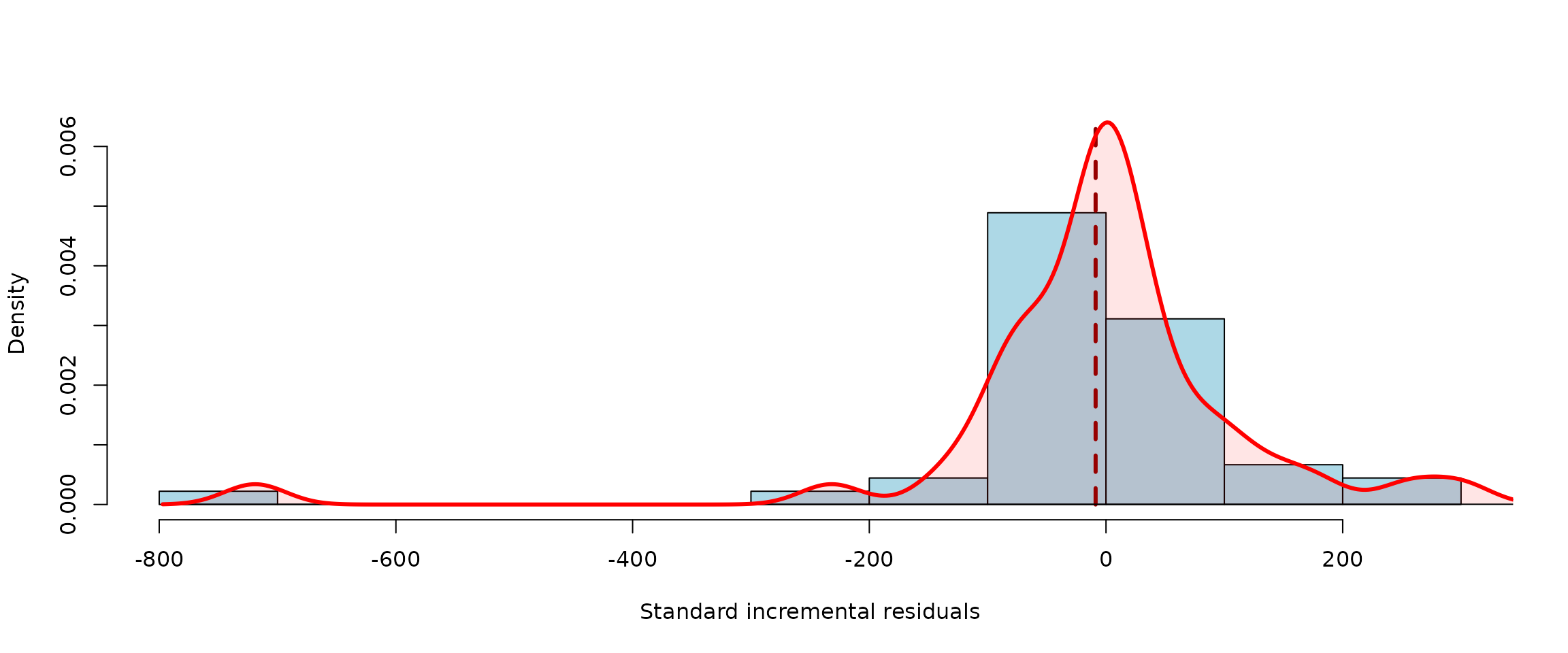

Unlike the output from the PARALLAX algorithm, there is an additional information about the incremental residuals provided in the output from REACT. Residuals are typically used by actuaries to evaluate the performance of the prediction. The residuals are available from the corresponding list item $residulas (which is provided in the output—the object of the class profileLadder—if the residuals are selected, i.e., residuals = TRUE). The residuals are defined as differences between true incremental payments $X_{i,j}$ and the predicted ones _{i,j}$ and they can be also printed within the triangle as

react.cameron$residuals

##       dev
## origin  1    2    3   4    5    6   7   8   9  10
##     1  NA   NA   NA  NA   NA   NA  NA  NA  NA  NA
##     2  NA   NA   NA  NA   NA   NA  NA  NA  NA   2
##     3  NA   NA   NA  NA   NA   NA  NA  NA  20  42
##     4  NA   NA   NA  NA   NA   NA  NA -20  34  -1
##     5  NA   NA   NA  NA   NA   NA -40  -7  -3  22
##     6  NA   NA   NA  NA   NA   -3  99 -84  30 118
##     7  NA   NA   NA  NA  179  -70  25 -31 -73  -1
##     8  NA   NA   NA 300  255  -83  82 -92  -4   0
##     9  NA   NA    5 147   56  -65  87 -34  -4   1
##     10 NA -719 -232 -49 -139 -114  43 -69  -5   0

If there are no residuals provided in the output (i.e., residuals = FALSE) and the graphical option is set to plotOption = TRUE, then slightly different figure (with the prediction summary in terms of a barplot) is provided:

summary(parallelReserve(cameron, method = "react"), plotOption = TRUE)

## REACT reserve prediction (by origins)
##       First Latest Dev.To.Date Ultimate IBNR
## 2      5984  13113   1.0000000    13113    0
## 3      7452  15720   0.9997456    15724    4
## 4      7115  13872   0.9937675    13959   87
## 5      5753  11282   0.9912142    11382  100
## 6      3937   8757   0.9725677     9004  247
## 7      5127   9325   0.9528919     9786  461
## 8      5046   8984   0.9172963     9794  810
## 9      5129   8202   0.8210210     9990 1788
## 10     3689   3689   0.4314620     8550 4861
## total 49232  92944   0.9174942   101302 8358

## Overall reserve summary

##     Est.Reserve    Est.Ultimate     Paid Amount    True Reserve        Reserve% 
##         8358.00       113517.00       105159.00         7963.00            4.96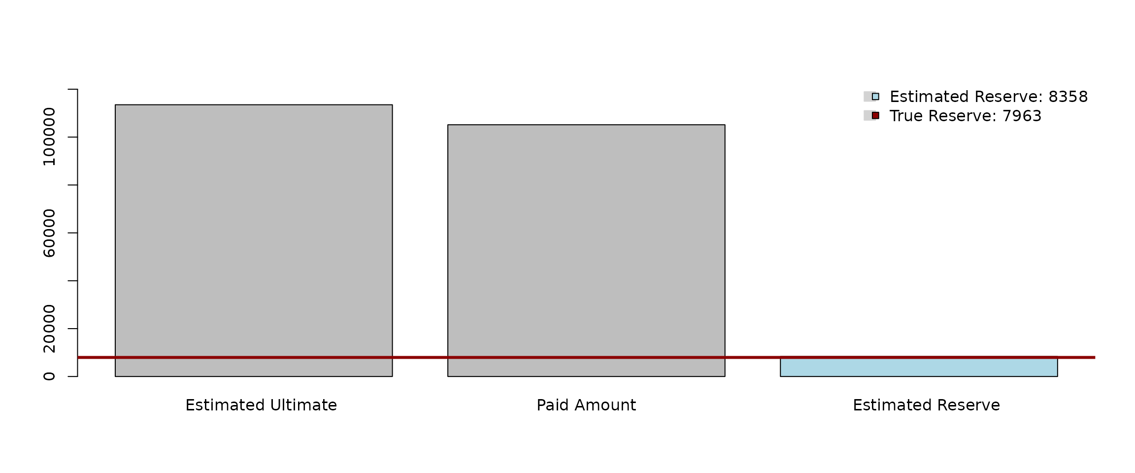

Note: There are two sets of residuals typically used by actuaries and both of them can be provided in the output of the parallelReserve() function. Either standard residuals in terms of $X_{i,j} - \widehat{X}_{i,j}$ are provided if the “future” (unknown) increments are available (for instance, for some retrospective back-testing or validation purposes) or, alternatively, so-called “back-fitted” residuals are calculated instead.

The main idea behind the back-fitted residuals is to flip the completed triangle, transform it back to the run-off triangle by deleting the lower triangularpart, and to use such run-off triangle as an~input to back-predict the run-off triangle by applying the same estimation procedure in_areverse manner so to say. Formally, the flipped matrix is a transposition with respect to the second diagonal—mathematically expressed, for a completed square $\{\widehat{Y}_{i,j};~i = 1, \dots, n; j = 1, \dots, n\}$ , the “flipped triangle” is the square $\{\widetilde{Y}_{i,j};~i= 1, \dots, n; j = 1, \dots, n\}$ , where $\widetilde{Y}_{i,j} = \widehat{Y}_{n + 1 - i, n + 1 - j}$ .

For illustration, and differences between the standard incremental residuals and the back-fitted residuals (that are more common in claims reserving practice), compare the following two outputs:

### standard residuals for a fully observed square
parallelReserve(cameron, method = "react", residuals = TRUE)$residuals  

### backfitted residuals for the observed run-off triangle only
parallelReserve(observed(cameron), method = "react", residuals = TRUE)$residuals

4. MACRAME

The idea of the MACRAME algorithm (MArkov Chain fRAgMEnt approximation) is to utilize a homogeneous Markov chain (MC) model to obtain the reserve prediction. This strategy is slightly different and more complex than the previous two; despite its additional mathematical complexity, however, it is quite intuitive and can be seen as a complex but rigorous generalization of the previous two algorithms described above. The underlying stochastic model invites additional user-defined adjustments and practically oriented modifications.

Unlike the previous two algorithms, MACRAME is based on the incremental run-off triangle. In the first step, the algorithm transforms the incremental payments $\{X_{i,j}; i = 1, \dots, n; j = 1, \dots, n + 1 - i\}$ into a finite set of states of a homogeneous Markov chain, ${S} = \{s_1, \dots, s_m\}$ , and the observed run-off triangle is used to estimate the matrix of the corresponding transition probabilities $\mathbb{P} = \big(p(s_{\iota_1}, s_{\iota_2})\big)_{\iota_1 = 1, \iota_2 = 1}^{|{S}|, |{S}|}$ , for $p(s_{\iota_1}, s_{\iota_2}) = \mathsf{P}[U_{i, j + 1} = s_{\iota_2} | U_{i, j} = s_{\iota_1}]$ where the increment $X_{i, j}$ is represented by the Markov state from ${S}$ that is taken by $U_{i,j}$ . Thus, there are three pivots behind the MACRAME algorithm:

Break points – the set of points $- \infty = g_0 < g_1 < \dots < g_{m - 1} < g_m = \infty$ ;
Markov states – the set of points $S = \{s_1, \dots, s_m\}$ , where, typically, $m = n$ ;
Transition matrix – the matrix $\mathbb{P} = \big(p(s_{\iota_1}, s_{\iota_2})\big)_{\iota_1 = 1, \iota_2 = 1}^{|{S}|, |{S}|}$ with the corresponding estimates for the probabilities of transitions between the states.

The MACRAME algorithm is implemented in the R function mcReserve() (from the ProfileLadder package) using a similar scope as the parallelResrve() function discussed above. The run-off triangle completion and the reserve prediction obtained by the DEFAULT (data-driven) verion of the MACRAME algorithm can be obtained by running

(macrame.cameron <- mcReserve(cameron))

## MACRAME Reserving 
##     Estimated Reserve    Estimated Ultimate           Paid Amount 
##              8081.963            113240.963            105159.000 
##          True Reserve 
##              7963.000

## MACRAME method (functional profile completion)

## 5244      9228   10823   11352   11791   12082   12120   12199   12215   12215   
## 5984      9939   11725   12346   12746   12909   13034   13109   13113   13160   
## 7452     12421   14171   14752   15066   15354   15637   15720   15756   15799   
## 7115     11117   12488   13274   13662   13859   13872   13919   13960   14003   
## 5753      8969    9917   10697   11135   11282   11340   11380   11422   11464   
## 3937      6524    7989    8543    8757    8815    8855    8897    8939    8982   
## 5127      8212    8976    9325    9496    9588    9646    9693    9737    9780   
## 5046      8006    8984    9677   10157   10458   10641   10759   10840   10902   
## 5129      8202    9244    9808   10165   10376   10502   10586   10649   10701   
## 3689      4731    5295    5652    5863    5989    6073    6136    6188    6236

The output of the MACRAME algorithm is again the S3 class object profileLadder and, thus, the same S3 methods as before can be applied again (in particuler, the following S3 methods are available: print(), plot(), and summary()). The performance of all three nonparametric prediction algorithms (PARALLAX, REACT, and MACRAME) can be quantitatively and visually compared (using the Cameron Mutual dataset).

par(mfrow = c(1,3))

### PARALLAX reserve prediction and run-off completion
plot(parallelReserve(cameron))

### REACT reserve prediction and run-off completion
plot(parallelReserve(cameron, method = "react"))

### MACRAME reserve prediction and run-off completion
plot(mcReserve(cameron))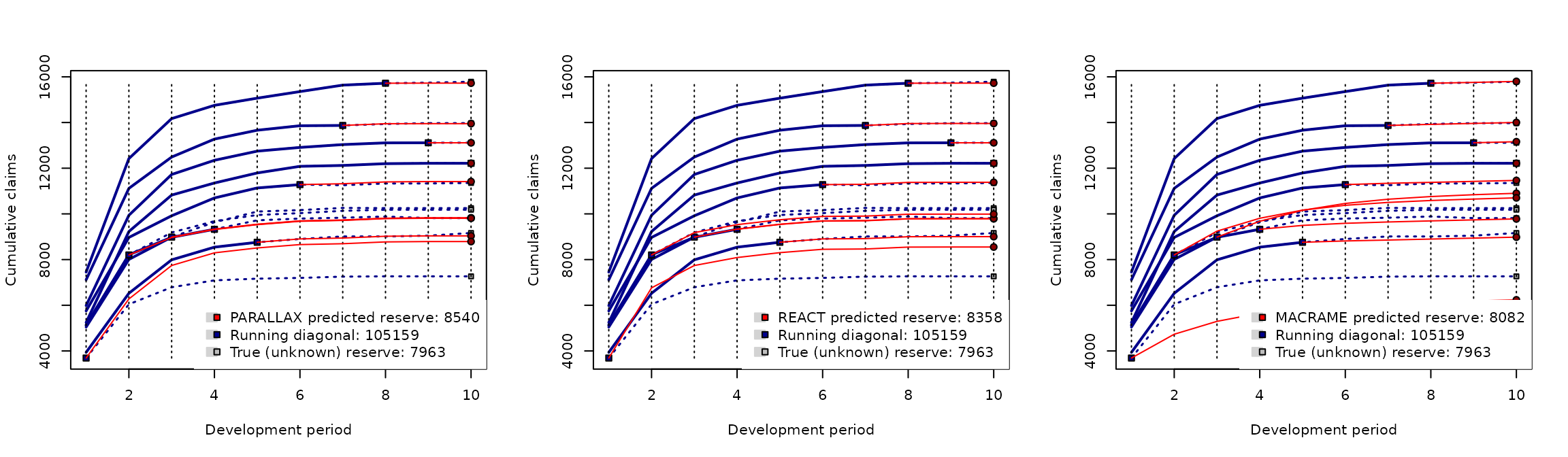

The red curve segments represent the predicted profile completions. The blue solid lines represent the available data—the underlyhing run-off triangle and the blue dotted lines stands for the “unknown” true developments (if available in the input data).

Recall, that the true reserve is $R = 7963$ . The reserve predictions provided by the proposed nonparametric reserving methods are

PARALLAX: $\widehat{R} = 8540$
REACT: $\widehat{R} = 8358$
MACRAME: $\widehat{R} = 8082$

This can be directly compared with the performance of some common parametric reserving methods implemented in the ChainLadder package:

chainladder method (implemented in chainladder()): $\widehat{R} = 8687$
over-dispersed Poisson model (glmReserve()): $\widehat{R} = 8601$
Tweedie model (tweedieReserve()): $\widehat{R} = 8610$

The best reserve prediction (in terms of the smallest difference between the true reserve) is given by the MACRAME algorithm. More complex empirical comparisons can be found in Maciak, Mizera, and Pešta (2022).

The underlying stochastic model behind the MACRAME algorithm invites additional user-defined adjustments and practically oriented modifications; unlike the MACRAME algorithm described in Maciak, Mizera, and Pešta (2022), where only a constrained and rather limited version of the algorithm was proposed, the implementation in the R function mcReserve() in the ProfileLadder package allows for all kinds of fine tuning and user-based modifications. Specific details can be either found in Maciak, Matúš, Mizera, and Pešta (2026) or in the package documentation (GitHub or CRAN).

Maciak, M., Mizera, I., and Pešta, M. (2022). Functional Profile Techniques for Claims Reserving. ASTIN Bulletin, 52(2), 449 – 482. DOI: 10.1017/asb.2022.4

Maciak, M., Matúš, R., Mizera, I., and Pešta, M. (2026). ProfileLadder: Functional-Based Reserving. The R journal, (to appear). URL: https://journal.r-project.org/issues.html

User-based modifications of MACRAME

The implementation of the algorithm in the R function mcReserve() allows users to intervene with various modifications—starting with a pre-specified
number of the Markov states to be required, selecting the method how the run-off triangle increments are summarized into the states, or providing a fully manual specification of the states ${S} = \{s_1, \dots, s_m\}$ , breaks $\{g_k\}_{k = 0}^m$ , or the subset of increments to be used.

Details (that are omitted here) can be found in the R help session for the mcReserve() function by typing

help("mcReserve")

In order to get some useful insight about the structure of the incremental run-off triangle and to offer some visual inspection for various user-based modifications of the underlying Markov chain in the mcReserve() function, there is another practical tool implemented in the ProfileLadder package—function incrExplor().

The function takes the run-off triangle as an input (fully observed or not, incremental or cumulative) and returns a complex empirical exploration of the incremental payments (that are used by macrame() to set the Markov chain within the MACRAME algorithm).

The default performance of the incrExplor() function returns a fully data-driven setup of the underlying Markov chain—the set of the data-driven Markov states and the corresponding set of break points:

(exploratory.casco <- incrExplor(casco))

## Data-driven (default) setting of the Markov Chain in MACRAME

## MC States: -957.5 -272 -129.5 -90 -55.5 -35.5 -25.5 -13 -4 0 230.5 420 716.5 1645 3863 116245 172120.5
## 
## Corresponding bins for the run-off triangle increments
##  [1] "[-Inf, -390)"    "[-390, -162)"    "[-162, -98)"     "[-98, -69)"     
##  [5] "[-69, -43)"      "[-43, -30)"      "[-30, -18)"      "[-18, -6)"      
##  [9] "[-6, 0)"         "[0, 123)"        "[123, 299)"      "[299, 489)"     
## [13] "[489, 1239)"     "[1239, 2725)"    "[2725, 98941)"   "[98941, 146134)"
## [17] "[146134, Inf)"

The output from the incrExplor() function is an object of the S3 class mcSetup and the S3 methods summary() and plot() can be applied to get further details.

summary(exploratory.casco)

## Input triangle type: Cumulative

## Summary of the increments
##                        Min   1st Q. Median       Mean   3rd Q.    Max
## Raw increments  -3028.0000 -62.0000     -2 18235.0000 867.0000 256454
## Std. increments    -0.0118  -0.0002      0     0.0711   0.0034      1
##                    Std.Er.
## Raw increments  51534.0000
## Std. increments     0.2009
## 
## Total number of increments: 136,  Total number of unique increments: 121
## Number of suspicious increments (using 2σ rule): 15,  Outliers (3σ rule): 6
## 
## Data-driven bins for the run-off triangle increments
##  [1] "[-Inf, -390)"    "[-390, -162)"    "[-162, -98)"     "[-98, -69)"     
##  [5] "[-69, -43)"      "[-43, -30)"      "[-30, -18)"      "[-18, -6)"      
##  [9] "[-6, 0)"         "[0, 123)"        "[123, 299)"      "[299, 489)"     
## [13] "[489, 1239)"     "[1239, 2725)"    "[2725, 98941)"   "[98941, 146134)"
## [17] "[146134, Inf)"  
## 
## Markov Chain states (medians of the increments within each bin)
##  [1]   -957.5   -272.0   -129.5    -90.0    -55.5    -35.5    -25.5    -13.0
##  [9]     -4.0      0.0    230.5    420.0    716.5   1645.0   3863.0 116245.0
## [17] 172120.5

plot(exploratory.casco)

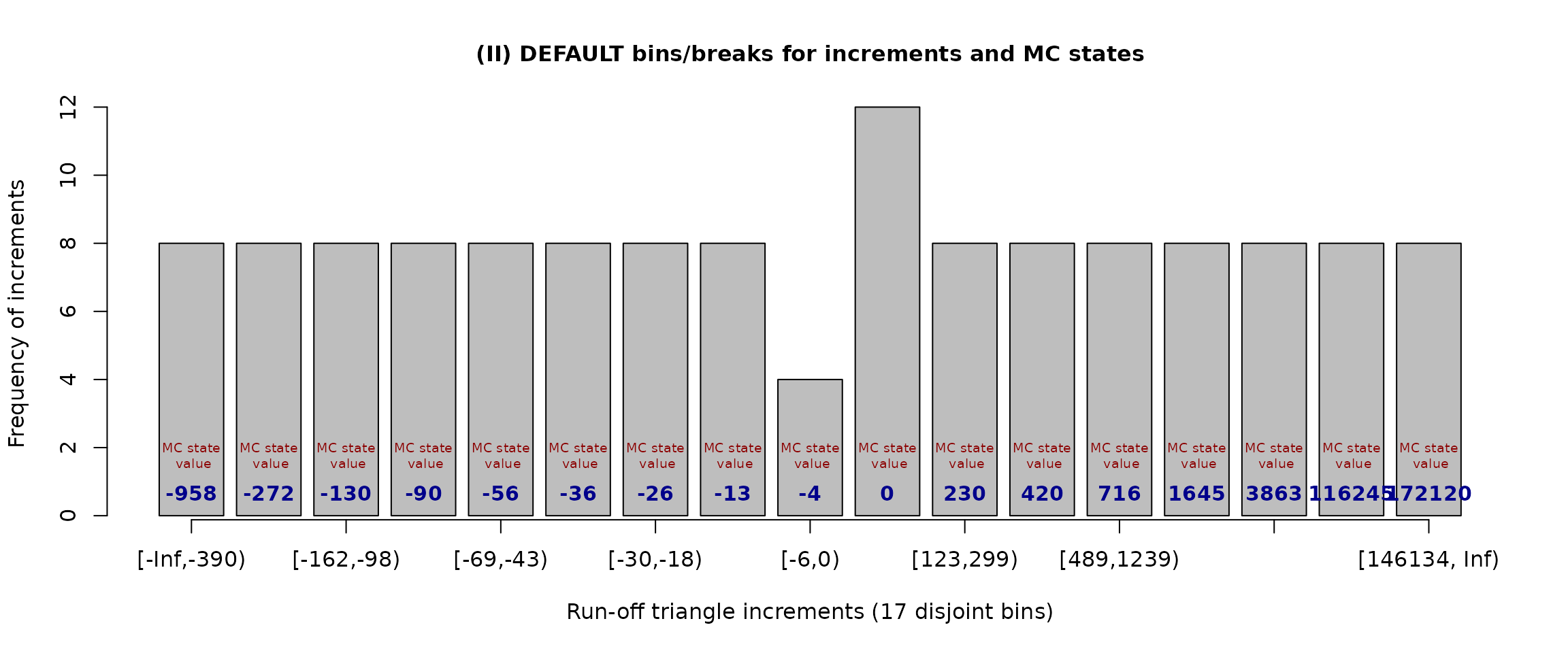
Using the barplot figure above, the break-points $\{g_{m}\}_{m = 0}^n$ are listed as interval labels on the $x$ axis. The Markov states (taken by default as medians of the increments belonging to a specific interval defined by two consecutive break points) are given as the blue labes within the bars.

The data-driven method for defining the break points and the corresponding Markov states (that are provided in the outputs above) is described and theoretically justified in Maciak, Mizera, and Pešta (2022). Further details are omiited here.

Possible user-based modifications are described in the following sections.

a) Modifying the underlying Markov states

It can be noticed from the barplot above that there are relatively many small (negative) Markov states (-957.5, -272.0, -129.5, etc.) that are due to many rather small negative increments while there are much more important (from the reserve prediction point of view) and much larger positive claim payments that are reflected in a roughly same amount of positive Markov states.

Thus, it could be interesting to modify the underlying Markov chain in a way that all negative increments are rather ignored—for instance, by introducing just one state for all zero and negative payments—and to focuss more on crutial claim payments that may heavily effect the final reserve. This can be done by the additional parameter states = ... which is implemented in both functions—the exploratory function incrExplor() and the prediction algorithm mcReserve().

In the following outputs, there are eight explicit Markov states used (c(0, 230, 420, 716, 1645, 3863, 116245, 172120)) and the corrresponding break points $g_1 < ... < g_{7}$ are determined as middle points between two consecutive Markov states (with $g_0 = -\infty$ and $g_9 = \infty$ ):

plot(modification.1 <- incrExplor(casco, states = c(0, 230, 420, 716, 1645, 3863, 116245, 172120)))

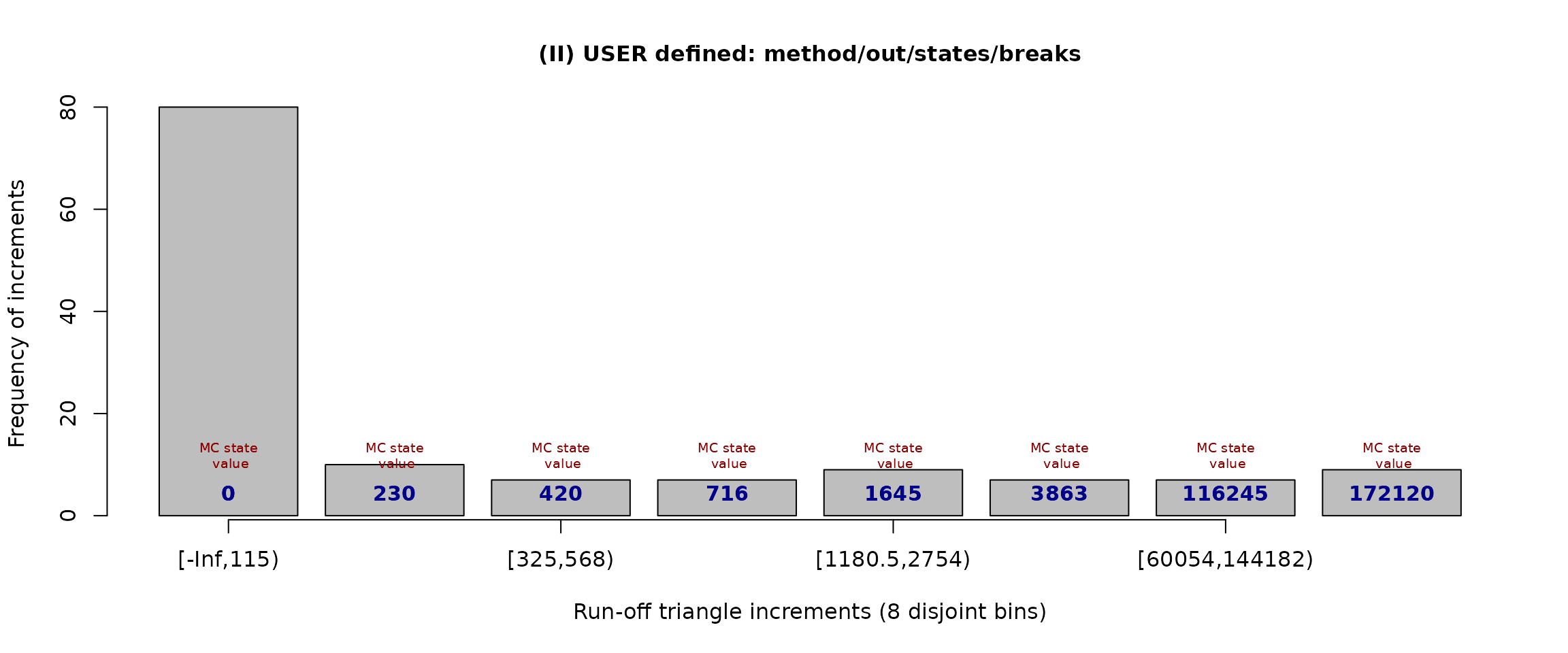
The same set of Markov states can be analogously used to run the MACRAME prediction (the output is omitted for brevity):

mcReserve(casco, states = c(0, 230, 420, 716, 1645, 3863, 116245, 172120))

All negative and small (i.e., below $115$ ) increments are now represented by one Markov state (zero) and other incremental payments are represented by the remaining seven pre-specified states. The MACRAME prediction with the same set of states can be performed by the mcReserve() function by using the dedicated accesor method mcStates() as follows (alternatively, the sequence of the states can be also plugged in explicitly):

mcReserve(casco, states = mcStates(modification.1))

The run-off triangle incremental payments are no longer equally distributed among the bins—this can be only achieved if the break points are calculated in the proposed data-driven manner.

However, the states parameter can be also specified differently. Instead of specifying the underlying set of the Markov states it can be used to change the amount of the states. For instance, the choice states = 5 will result in five Markov states and, again, the increments will be distributed equally (as much as possible). This can be also verified visually by

plot(incrExplor(casco, states = 5))

The same Markov states (rounded in the figure above) will be used by the MACRAME algorithm when specifying the same amount of the Markov states, i.e., state = 5. This can be directly veryfied by the following:

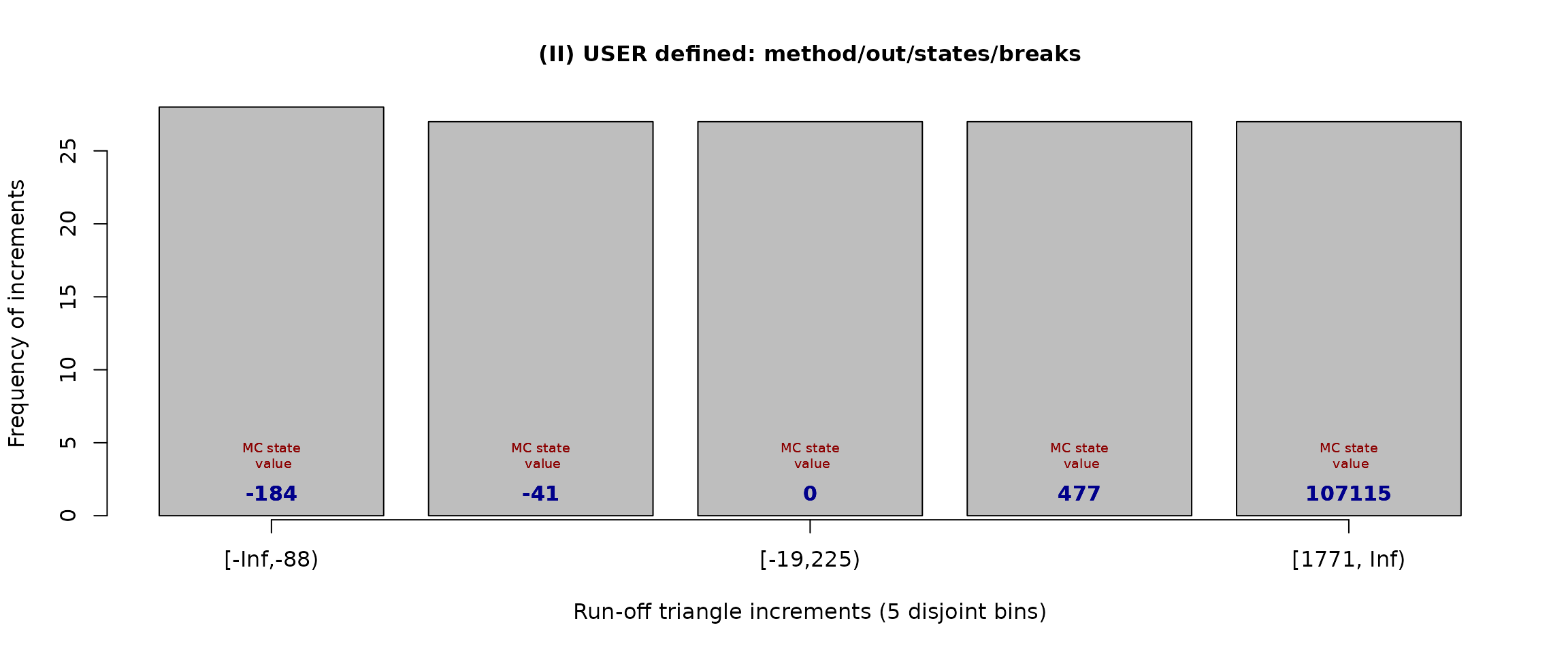
macrame.s5.casco <- mcReserve(casco, states = 5)
mcStates(macrame.s5.casco)

## [1]   -184.5    -41.0      0.0    477.0 107115.0

The corresponding break points are

mcBreaks(macrame.s5.casco)

## [1] -Inf  -88  -19  225 1771  Inf

and the transition matrix with the estimated transition probabilities is

mcTrans(macrame.s5.casco)

##        [,1]   [,2]   [,3]   [,4]   [,5]
## [1,] 0.2801 0.1960 0.3839 0.1400 0.0000
## [2,] 0.1644 0.2959 0.4740 0.0658 0.0000
## [3,] 0.0000 0.0000 1.0000 0.0000 0.0000
## [4,] 0.2206 0.1575 0.3383 0.1890 0.0945
## [5,] 0.1315 0.0000 0.2767 0.3288 0.2630

b) Specifying explict break points

Another parameter implemented for user modifications of the Markov chain in the MACRAME algorithm is the parameter breaks which can be used to explicitly provide the set of break points for the run-off triangle increments.

However, a valid sequence of the break points—in a sense that $g_1 < g_2 < \dots < g_{m - 1}$ —must be provided. The first and the last break point ( $g_0 = - \infty$ and $g_m = \infty$ ) may or may not be specified. On the other hand, two consecutive break points always need to contain at least one incremental payment in between—otherwise, such consecutive bins are merged together to form a new one.

Going back to the Casco incurance data where many negative increments were noticed, it can be more appropriate to alter the underlying Markov chain by providing a different set of break points (rather than changing directly the Markov states). In such a way, the corresponding Markov states will be still obtained using a statistical summary method (by default, the Markov states are medians of the increments within the bins).

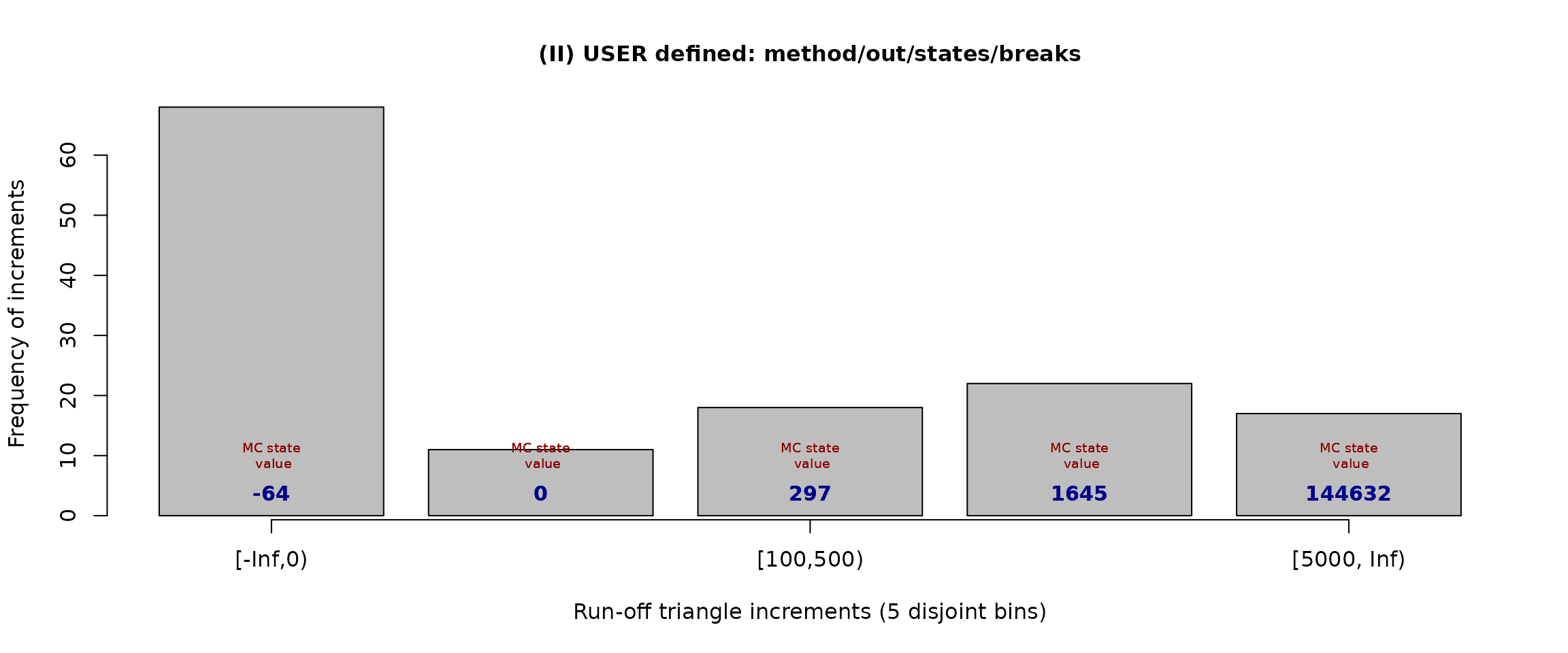
The default break points are determined in a way that the increments are equaly distributed among 17 non-overlapping bins (where the number of bins being used is, by default, same as the dimension of the run-off triangle). For instance, five bins with explicit breaks points $\{g_{m}\}_{m = 0}^5 \equiv \{-\infty, 0, 100, 500, 5000, \infty\}$ can be obtained by

plot(modification.2 <- incrExplor(casco, breaks = c(0, 100, 500, 5000)))

and the same resuld will be also obtained for any of the following (outputs are omitted):

incrExplor(casco, breaks = c(-Inf, 0, 100, 500, 5000))
incrExplor(casco, breaks = c(0, 100, 500, 5000, Inf))
incrExplor(casco, breaks = c(-Inf, 0, 100, 500, 5000, Inf))

The corresponding Markov states are calculated (by default) as medians of the increments within each bin and they can be assessed by using the mcStates() function

mcStates(modification.2)

## [1]    -63.5      0.0    297.0   1645.0 144632.0

The corresponding MACRAME reserve prediction using the same break points (and the corresponding Markov states as well) is obtained analogously by

summary(mcReserve(casco, breaks = c(0, 100, 500, 5000)))

## MACRAME reserve prediction (by origins)
##          First   Latest Dev.To.Date   Ultimate       IBNR
## 2       423582   522003   0.9999172   522046.2    43.2500
## 3       373866   485984   1.0000000   485984.0     0.0000
## 4       441769   557049   0.9996132   557264.5   215.5362
## 5       503292   630271   1.0000000   630271.0     0.0000
## 6       554625   701433   1.0000000   701433.0     0.0000
## 7       613011   758233   0.9993793   758703.9   470.9047
## 8       605922   761068   0.9992867   761611.3   543.2598
## 9       555154   670158   0.9988864   670905.1   747.1026
## 10      514900   626112   0.9965579   628274.6  2162.6048
## 11      581196   708428   0.9988083   709273.2   845.2127
## 12      613266   781561   0.9990129   782333.3   772.2756
## 13      706120   894514   0.9973982   896847.4  2333.3986
## 14      859707  1059593   0.9977591  1061972.8  2379.7958
## 15      951189  1207771   0.9891633  1221002.6 13231.6383
## 16     1061511  1317965   0.9900306  1331236.6 13271.6275
## 17     1121591  1121591   0.9882740  1134898.8 13307.8470
## total 10480701 12803734   0.9960849 12854058.5 50324.4536

## Overall reserve summary

##     Est.Reserve    Est.Ultimate     Paid Amount    True Reserve        Reserve% 
##        50324.45     13543555.45     13493231.00              NA              NA

c) Summary method for incremental payments

Instead of summarizing the increments within each bin by considering the median value, another method can be specified by another parameter method which can take on of four values: "median" (default); "mean", "min", and "max".

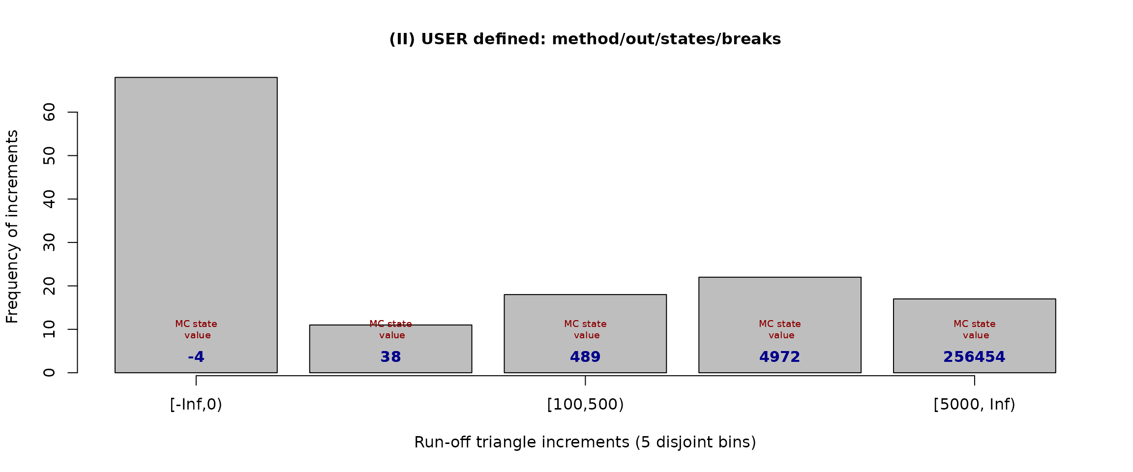
Thus, considering the same set of breaks as before, it can be of some interest to define Markov states not as medians of the increments within each bin but taking maximum in every bin instead. This can be easily achieved by

new.breaks <- c(0, 100, 500, 5000)
exploratory.casco2 <- incrExplor(casco, breaks = new.breaks, method = "max")
plot(exploratory.casco2)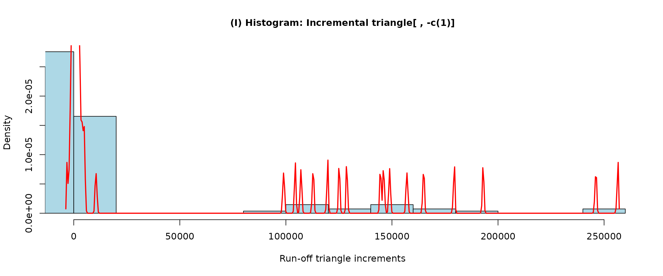

The parameter method is only available for the exploratory function incrExplor() and, unlike the parameters states and breaks, it is not implemented in the mcReserve() function. This is, however, not limiting with respect to the performance of the MACRAME algorithm implemented within mcReserve(). Indeed, the parameter method = c("median", "mean", "min", "max") is used to summarize the increments within each bin defined by the break points in breaks = ... and the corresponding Markov states can be assessed from the incrExplor() function by using the appropriate accessor method, the function mcStates(). Consequently, both the breaks (provided explicitly) and the states (obtained as maximal increments within each bin) can be forwarded into the mcReserve() function to set up the MACRAME algorithm correspondingly (output is omitted again):

mcReserve(casco, breaks = mew.breaks, states = mcStates(exploratory.casco2))

The previous also implies that users can fully manually set the breaks and the Markov states when running the MACRAME algorithm. A valid set of breaks is needed and the states must be always provided in a way, that exactly one Markov state belongs to one interval determined by two consecutive break points. More details can be found the package documentation—particularly in the following two help sessions

help("incrExplor")
help("mcReserve")

Note: There are four parameters implemented in the incrExplor() function to help users to properly tune the underlying Markov chain for the MACRAME prediction (breaks = ..., states = ..., method = ..., and out = ...). On the other hand, there are only two parameters used within the mcReserve() function.

The summary method for run-off triangle increments can be enforced within the mcReserve() function by using the appropriate accessor functions:

mcBreaks() – function for extracting the set of break points from incrExplor() or mcReserve();
mcStates() – function for extracting the Markov states from incrExplor() or mcReserve();
mcTrans() – function to extract the estimated transition matrix from mcReserve().

Note that the mcTrans() function can be only applied to the output of the mcReserve() function as there is not transition probability estimation in the exploratory tool incrExplor().

The parameter out = ... implemented in the incrExplor() function is discussed in the next section.

d) Subsets of incremental payments

The default functionality of the incrExplor() function is to provide users with the data-driven set of bins (the break points respectively) and the corresponding Markov states for the underlying run-off triangle. The first year payments in the run-off triagnle are not considered by default (further discussion is provided in Maciak, Mizera, and Pešta, 2022), but this restriction can be also altered—if needed.

If there is a specific interest to also include the first year payments when defining the Markov chain states and the corresponding break points (or, alternatively, to exclude some other columns with the incremental payments), an additional parameter out = 1 (default) can be changed correspondingly—the default value stands for the first year increments that are typically not considered; the choice out = 0 uses all available increments $X_{i,j}$ , for $i = 1, \dots, n$ and $j = 1, \dots, n + 1 - i$ ; in order to exclude, for example, first three columns, the parameter can be specified as out = c(1,2,3). The change of this parameter is also reflected by the output of incrExplor() which, in addition, contains analogous information as before, however, for a user-modified subset of the incremental payments.

incrExplor(cameron, out = 0)

## Data-driven (default) setting of the Markov Chain in MACRAME

## MC States: 13 81 197 302.5 438 601 948 1672.5 3073 3993
## 
## Corresponding bins for the run-off triangle increments
##  [1] "[-Inf, 75)"   "[75, 147)"    "[147, 288)"   "[288, 388)"   "[388, 554)"  
##  [6] "[554, 780)"   "[780, 1465)"  "[1465, 2587)" "[2587, 3955)" "[3955, Inf)"

## User-modified MC setting

## MC States: 14.5 125 285.5 400 601 978 2186.5 3689 5007.5 5984
## 
## Corresponding bins for the run-off triangle increments
##  [1] "[-Inf, 79)"   "[79, 197)"    "[197, 349)"   "[349, 529)"   "[529, 786)"  
##  [6] "[786, 1595)"  "[1595, 3085)" "[3085, 3984)" "[3984, 5244)" "[5244, Inf)" 
## 
## Development periods (run-off triangle columns) not considered: 0
## Method selected to summarize the increments within each bin: DEFAULT (median)

The S3 method plot() can be applied to obtain some graphical visualization of the user-defined subset of increments and their overall summary (together with the comparison with the default selection).

par(mfrow = c(1,2))
plot(incrExplor(cameron, out = 0))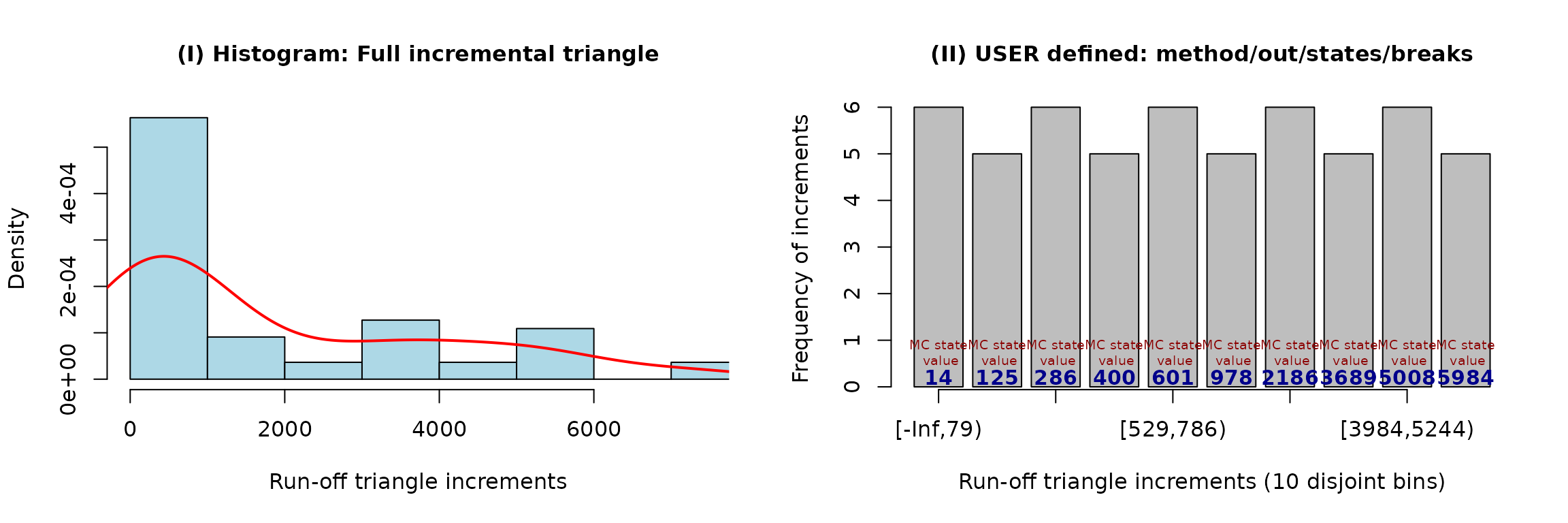

e) Illustration of different MACRAME settings

Different settings for the break points and the Markov states result in different reserve predictions (and the corresponding missing profiles completions). In the following, there is again the Cameron Mutual dataset used (with the known true reserve 7963) with the predicted reserves ranging from 7827 (slightly underestimated reserve) up to 22587 (heavily overestimated reserve).

Various user-based modifications are used for the MACRAME predictions below (the first one being the default performance).

par(mfrow = c(3,2))

plot(mcReserve(cameron)) ### default setting with 10 MC states
plot(mcReserve(cameron, states = 4)) ### four states (otherwise default)
plot(mcReserve(cameron, states = c(50, 500, 1500, 3000))) ### explicit states
plot(mcReserve(cameron, breaks = c(500, 1000, 1500, 2000))) ### explicit breaks
     
user.breaks <- c(500, 1000, 1500, 2000)
user.method <- incrExplor(cameron, breaks = user.breaks, method = "max")
final.states <- mcStates(user.method)
### explicit breaks and Markov states as maximma 
plot(mcReserve(cameron, breaks = user.breaks, states = final.states))

### explicit breaks and explicit states
plot(mcReserve(cameron, breaks = c(500, 1000, 1500), states = c(100, 999, 1001, 3000)))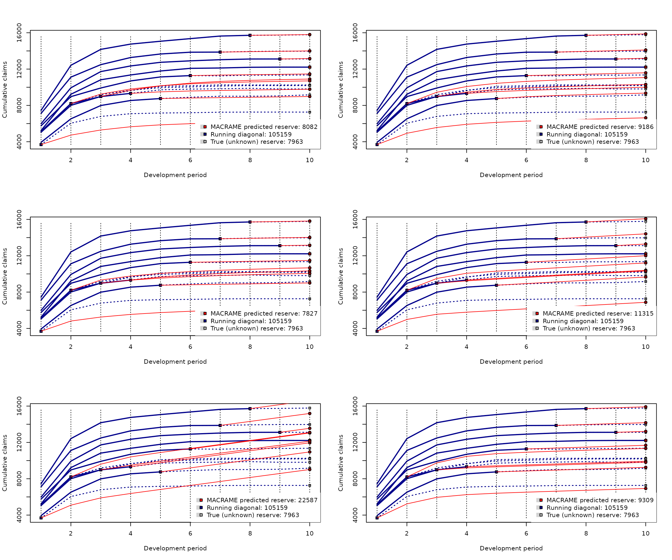

Note: The default performance of the MACRAME algorithm implemented by the R function mcReserve() is fully-data driven and it fully corresponds with the breaks and Markov states as proposed and theoretically justified in Maciak, Mizera, and Pešta, (2022).

5. Permutation bootstrap

The reserve prediction $\widehat{{R}}$ for the unknown claims reserve ${R}$ provides only a partial information in the entire loss reserving problem. In practice, a prediction of the whole reserve distribution is required too (for instance, by risk reserving assessment guidelines like Solvency II).

Classical techniques employ a residual (parametric or semiparametric) bootstrap approach (typically based on the back-fitted residuals) to emulate the distribution of interest. However, for the functional-based claims reserving there is a different strategy: permutation bootstrap. The prediction of the reserve distribution is still obtained via bootstrap resampling, but the algorithm avoids the use of residuals by resampling (permuting) the whole functional profiles. The rows of the completed run-off triangle produced by a certain algorithm—by each of those described above, but also any of the classical parametric reserving models implemented in the ChainLadder package—are treated as independent functional profiles. The completed triangle, the data matrix $\{\widehat{Y}_{i,j}\}_{i,j=1}^{n,n}$ , can be standardized: each row is divided by the first positive value within the row (considered from the left—which is, very likely, the first incremental payment in each row). The standardization step is proposed on the grounds that it is very typical in practice that the claims amounts paid in the first development period substantially increase over the years (possibly the effect of economical growth, inflation, more advanced or more expensive technology, etc.). The standardization is set as a default, but the user can suppress it if desiring so.

permute.cameron <- permuteReserve(mcReserve(cameron), B = 100)

The output from the permuteReserve() function is an object of the S3 class permutedReserve and S3 methods summary() or plot() can be applied to get more detailed information:

summary(permute.cameron)

## MACRAME based reserve prediction (with B = 100 bootstrap permutations)
##       First Latest Dev.To.Date   Ultimate       IBNR        S.E        CV
## 2      5984  13113   0.9964286  13160.000   47.00000   20.35946 0.4331799
## 3      7452  15720   0.9950067  15798.889   78.88889   38.10804 0.4830597
## 4      7115  13872   0.9906724  14002.611  130.61111  116.55286 0.8923656
## 5      5753  11282   0.9840866  11464.438  182.43827  158.73832 0.8700933
## 6      3937   8757   0.9749940   8981.594  224.59362  125.88048 0.5604811
## 7      5127   9325   0.9535135   9779.620  454.61986  253.74400 0.5581455
## 8      5046   8984   0.8241040  10901.537 1917.53724  552.09226 0.2879174
## 9      5129   8202   0.7664369  10701.468 2499.46806  644.56539 0.2578810
## 10     3689   3689   0.5915835   6235.806 2546.80632  523.25414 0.2054550
## total 49232  92944   0.9200011 101025.963 8081.96337 1348.35146 0.1668346

## Overall reserve distribution

##      Boot.Mean        Std.Er.       BootCov%    BootVar.995 
##    9526.563369    1348.351459      14.153598       1.436145 
## 
## The MACRAME predicted reserve represents the 10.89% quantile of the reserve distribution
## Bootstrap simulated reserves beyond 2σ rule: 5 (out of 100)

plot(permute.cameron)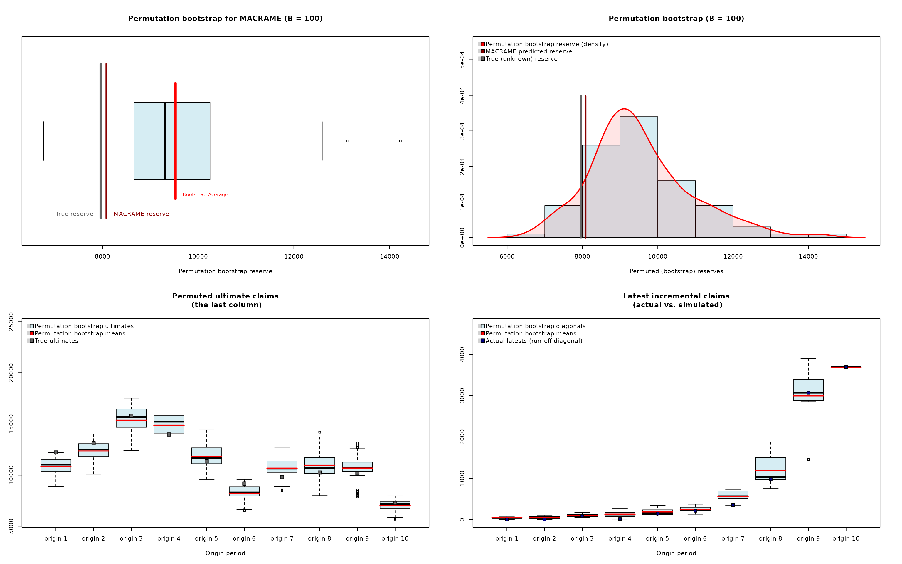

Note that in the summary output above there already colums S.E. and CV provided and they can be directly compared with the values obtained from the distributional assumption (using, for instance, the over-dispersed Poisson model) from the ChainLadder package

summary(glmReserve(observed(cameron)))

##       Latest Dev.To.Date Ultimate IBNR          S.E        CV
## 2      13113   1.0000000    13113    0   0.01035287       Inf
## 3      15720   0.9992372    15732   12  29.38975320 2.4491461
## 4      13872   0.9934116    13964   92  73.46098788 0.7984890
## 5      11282   0.9850694    11453  171  96.26787355 0.5629700
## 6       8757   0.9688019     9039  282 120.58781735 0.4276164
## 7       9325   0.9397360     9923  598 177.57019068 0.2969401
## 8       8984   0.8905630    10088 1104 246.00693847 0.2228324
## 9       8202   0.7789914    10529 2327 379.54811405 0.1631062
## 10      3689   0.4788422     7704 4015 622.22022041 0.1549739
## total  92944   0.9152986   101545 8601 880.66723938 0.1023913

Note: The permutation bootstrap implemented in the R function permuteReserve() (from the R package ProfileLadder) handles not only objects created by the parallelReserve() function and the mcReserve() function (thus, S3 objects of the class profileLadder) but it also works with the objects generated by the classical reserving techniques—those implemented in the R package ChainLadder (in particular, the over-dispersed Poisson model, the Mack model, chainladder model, or the Tweedie formula).

Note also the same layout used for the S3 method plot() when applied to the output of the permutation bootstrap function pemuteReserve() as the one adoped for the residual bootstrap resampling in classical parametric chainladder based methods:

plot(BootChainLadder(observed(cameron)))

Thus, the overall distributional (reserve) prediction can be obtained from different perspective: adopting some distributional assumptions (such as the Poisson model), using the residual bootstrap approach, or performing the permutation bootstrap for whole functional profiles.

cameron.glm <- glmReserve(observed(cameron))
cameron.boot <- glmReserve(observed(cameron), mse.method = "bootstrap", nsim = 100)
cameron.permute <- permuteReserve(glmReserve(observed(cameron)), B = 100)

All three summary() outputs below contains full information (especially the last two columns denoted as S.E and CV):

summary(cameron.glm)

##       Latest Dev.To.Date Ultimate IBNR          S.E        CV
## 2      13113   1.0000000    13113    0   0.01035287       Inf
## 3      15720   0.9992372    15732   12  29.38975320 2.4491461
## 4      13872   0.9934116    13964   92  73.46098788 0.7984890
## 5      11282   0.9850694    11453  171  96.26787355 0.5629700
## 6       8757   0.9688019     9039  282 120.58781735 0.4276164
## 7       9325   0.9397360     9923  598 177.57019068 0.2969401
## 8       8984   0.8905630    10088 1104 246.00693847 0.2228324
## 9       8202   0.7789914    10529 2327 379.54811405 0.1631062
## 10      3689   0.4788422     7704 4015 622.22022041 0.1549739
## total  92944   0.9152986   101545 8601 880.66723938 0.1023913

summary(cameron.boot)

##       Latest Dev.To.Date Ultimate IBNR       S.E         CV
## 2      13113   1.0000000    13113    0   0.00000        NaN
## 3      15720   0.9992372    15732   12  39.78803 3.31566877
## 4      13872   0.9934116    13964   92  69.63145 0.75686361
## 5      11282   0.9850694    11453  171  88.73998 0.51894727
## 6       8757   0.9688019     9039  282 108.17280 0.38359149
## 7       9325   0.9397360     9923  598 174.12157 0.29117319
## 8       8984   0.8905630    10088 1104 267.14475 0.24197894
## 9       8202   0.7789914    10529 2327 393.02842 0.16889919
## 10      3689   0.4788422     7704 4015 556.93632 0.13871390
## total  92944   0.9152986   101545 8601 841.41341 0.09782739

summary(cameron.permute)

## GLM based reserve prediction (with B = 100 bootstrap permutations)
##       First Latest Dev.To.Date Ultimate IBNR         S.E        CV
## 2      5984  13113   1.0000000    13113    0    0.000000       NaN
## 3      7452  15720   0.9992372    15732   12    3.087699 0.2573083
## 4      7115  13872   0.9934116    13964   92   14.070626 0.1529416
## 5      5753  11282   0.9850694    11453  171   35.269466 0.2062542
## 6      3937   8757   0.9688019     9039  282   89.645139 0.3178906
## 7      5127   9325   0.9397360     9923  598  140.511467 0.2349690
## 8      5046   8984   0.8905630    10088 1104  220.787040 0.1999883
## 9      5129   8202   0.7789174    10530 2328  544.173060 0.2337513
## 10     3689   3689   0.4789043     7703 4014 1225.273638 0.3052500
## total 49232  92944   0.9152986   101545 8601 1231.636024 0.1431968

## Overall reserve distribution

##      Boot.Mean        Std.Er.       BootCov%    BootVar.995 
##   10916.062751    1231.636024      11.282786       1.232687 
## 
## The GLM predicted reserve represents the 4.95% quantile of the reserve distribution
## Bootstrap simulated reserves beyond 2σ rule: 1 (out of 100)

Note: The permuteReserve() function returns a relatively complex R object of the S3 class permutedReserve which can be quite memory demanding (especially for large run-off triangles and large number of permutations. For this reason, there is an additional parameter outputAll = TRUE (set as TRUE by default) used to suppress compex outputs and important summary characteristics are printed only (for outputAll = FALSE).

6. Generic S3 method `predict()`

Finally, there is one key S3 method implemented in the R package ProfileLadder that was not mentioned yet—the S3 method predict(). This function is not only useful for the actuaries, but it also has important practical utilizations in any type of risk modeling. The S3 method predict() is implemented for the objects of the S3 class profileLadder that are created by the parallelReserve() function or the mcReserve() function (for details, we refer to the help session obtained by help("predict.profileLadder").

Instead of completing the run-off triangle into a full square (as performed by one of the algorithms PARALLAX, REACT, or MACRAME), the predict() method only returns the prediction of the next running diagonal (also called a 1-step-ahead prediction in the acturial circles).

The same nonparametric algorithms are used for the diagonal prediction; however, the output is not a completed square but rather a new (extended) run-off triangle of the dimensions $n \times (n + 1)$ :

(diag.cameron <- predict(parallelReserve(cameron)))

## 5244      9228   10823   11352   11791   12082   12120   12199   12215   12215   12215   
## 5984      9939   11725   12346   12746   12909   13034   13109   13113   13113       .   
## 7452     12421   14171   14752   15066   15354   15637   15720   15724       .       .   
## 7115     11117   12488   13274   13662   13859   13872   13947       .       .       .   
## 5753      8969    9917   10697   11135   11282   11320       .       .       .       .   
## 3937      6524    7989    8543    8757    8904       .       .       .       .       .   
## 5127      8212    8976    9325    9539       .       .       .       .       .       .   
## 5046      8006    8984    9333       .       .       .       .       .       .       .   
## 5129      8202    8966       .       .       .       .       .       .       .       .   
## 3689      6276       .       .       .       .       .       .       .       .       .

The S3 method plot() can be used to visualize the diagonal 1-step-ahead prediction

plot(diag.cameron)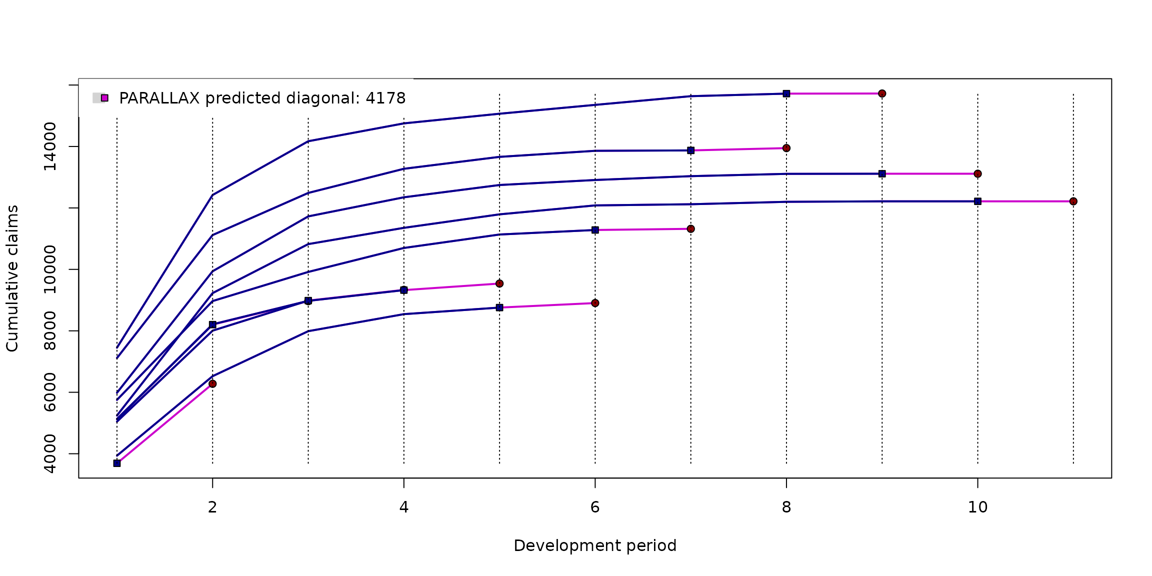

Conclussion

The main core of the R package ProfileLadder consists of three key functions—parallelReserve() for applying the PARALLAX or REACT algorithm, mcReserve() implementing the MACRAME algorithm, and permutedReserve() providing the permutation bootstrap add-on. Another generic functions (for the S3 objects of the class profileLadder, profilePredict, mcSetup, and permutedReserve) are also implemented to facilitate a well structured summary of the outputs and graphical visualizations of the results.

There are also a few other helpful functions implemented in the ProfileLadder package. For a complex description and illustrative examples, we refer to the R help sessions by using the standard help() command.

The ProfileLadder package is particularly developed to implement nonparametric methods into the actuarial risk assessment process performed by insurance companies (typically on a yearly or quarterly basis). Nevertheless, the underlying run-off triangle can be formally also represented in terms of an incomplete panel data scheme that is generally well known among statisticians and all types of practitioners.

Acknowledgement

The authors express sincere thanks to Kurt Hornik and Rob Hyndman for their insight and some useful pieces of advice regarding the ProfileLadder package. The authors are also grateful to Petr Jedlička from the Czech Insurers’ Bureau and Pavel Koudelka from Generali Česká pojišťovna a.s., for providing complex data from real-life insurance practice—not only for internal evaluation purposes but also for public access within the R package ProfileLadder.

Matúš Maciak, Rastislav Matúš, Ivan Mizera, and Michal Pešta